Chapter 2 Getting Hands on with Bayes Theorem

Bayesian inference is built on a different way of thinking about parameters of probability distributions than methods you have learnt so far. In the past 30 years or so, Bayesian inference has become much more popular. This is partly due to increased computational power becoming available. In this first section, we are going to set out to answer:

What are the fundamental principles of Bayesian inference?
What makes Bayesian inference different from other methods?
How do we carry out Bayesian inference in practice?

2.1 Statistical Inference

The purpose of statistical inference is to “draw conclusions, from numerical data, about quantities that are not observed” (Bayesian Data Analysis, chapter 1). Generally speaking, there are two kinds of inference:

Inference for quantities that are unobserved or haven’t happened yet. Examples of this might be the size of a payout an insurance company has to make, or a patients outcome in a clinical trial had they been received a certain treatment.
Inference for quantities that are not possible to observe. This is usual because they are part of modelling process, like parameters in a linear model.

In this module, we are going to look at a different way of carrying out statistical inference, one that doesn’t depend on long run events. Instead, we’re going to introduce the definition of probability that allows us to interpret the subjective chance that an event occurs.

2.2 Frequentist Theory

Frequentist probability is built upon the theory on long run events. Probabilities must be interpretable as frequencies over multiple repetitions of the experiment that is being analysed, and are calculated from the sampling distributions of measured quantities.

Definition 2.1 The long run relative frequency of an event is the probability of that event.

Example 2.1 If a frequentist wanted to assign a probability to rolling a 6 on a particular dice, then they would roll the dice a large number of times and compute the relative frequency.

Definition 2.2 A statistical model is a mathematical description of the assumptions about how observed data \(\boldsymbol{y}\) are generated. It specifies a relationship between the data and one or more unknown parameters \(\theta\).

The most common way to estimate the value of \(\theta\) is using maximum likelihood estimation. Although other methods do exist (e.g. method of moments, or penalised maximum likelihood estimation).

Definition 2.3 The maximum likelihood estimate of \(\theta\), \(\hat{\theta}\), is the value such that \(\hat{\theta} = \max_{\theta} p(\boldsymbol{y}\mid \theta)\).

Uncertainty around the maximum likelihood estimate is based on the theory of long running events that underpin frequentist theory.

Definition 2.4 Let \(Y\) be a random sample from a probability distribution \(\theta\). A \(100(1-\alpha)%\) confidence interval for \(\theta\) is an interval \((u(Y), v(Y))\) such that \[ \mathbb{P}(u(Y) < \theta < v(Y)) = 1-\alpha \]

This means that if you had an infinite number of samples for \(Y\) and the corresponding infinite number of confidence intervals, then \(100(1-\alpha)\)% of them would contain the true value of \(\theta\). It does not mean that there is a \(100(1-\alpha)\) probability a particular interval contains the true value of \(\theta\).

Given that we want to understand the properties of \(\theta\) given the data we have observed \(\boldsymbol{y}\), then you might think it makes sense to investigate the distribution \(p(\theta \mid \boldsymbol{y})\). This distribution says what are the likely values of \(\theta\) given the information we have observed from the data \(\boldsymbol{y}\). We will talk about Bayes’ theorem in more detail later on in this chapter, but, for now, we will use it to write down this distribution \[ p(\theta \mid \boldsymbol{y}) = \frac{p(\boldsymbol{y} \mid \theta)p(\theta)}{p(\boldsymbol{y})}. \] This is where frequentist theory cannot help us, particularly the term \(p(\theta)\). Randomness can only come from the data, so how can we assign a probability distribution to a constant \(\theta\)? The term \(p(\theta)\) is meaningless under this philosophy. Instead, we turn to a different philosophy where we can assign a probability distribution to \(\theta\).

2.3 Bayesian Probability

The Bayesian paradigm is built around a different definition of probability. This allows us to generate probability distirbutuions for parameters values.

Definition 2.5 The subjective belief of an event is the probability of that event.

This definition means we can assign probabilities to events that frequentists do not recognise as valid.

Example 2.2 Consider the following:

The probability that I vote for the labour party at the next election
A photo taken from the James Watt telescope contains a new planet.
The real identify of Banksy is Robin Gunningham.

These are not events that can be repeated in the long run.

2.4 Conditional Probability

Before we derive Bayes’ theorem, we recap some important definitions in probability.

Definition 2.6 Given two events \(A\) and \(B\), the conditional probability that event \(A\) occurs given the event \(B\) has already occurred is \[ p(A \mid B) = \frac{p(A \textrm{ and } B)}{p(B)}, \] when \(p(B) > 0\).

Definition 2.7 Two events \(A\) and \(B\) are independent given event \(C\) if and only if \[ p(A \textrm{ and } B \mid C) = p(A \mid C)p(B \mid C).\]

2.5 Bayes’ Theorem

Now we have an understanding of conditional probability and exchangeability, we can put these two together to understand Bayes’ Theorem. Bayes’ theorem is concerned with the distribution of the parameter \(\theta\) given some observed data \(y\). It tries to answer the question: what does the data tell us about the model parameters?

Theorem 2.1 (Bayes) The distribution of the model parameter \(\theta\) given the data \(y\) is \[ p(\theta \mid y) = \frac{p(y \mid \theta)p(\theta)}{p(y)} \]

Proof. \[\begin{align} p(\theta \mid y) &= \frac{p(\theta, y)}{p(y)}\\ \implies p(\theta, y) &= p(\theta \mid y)p(y) \end{align}\] Analogously, using \(p(y \mid \theta)\) we can derive \[ p(\theta, y) = p(y \mid \theta)p(\theta) \] Putting these two terms equal to each other and dividing by \(p(y)\) gives \[ p(\theta \mid y) = \frac{p(y \mid \theta)p(\theta)}{p(y)} \]

There are four terms in Bayes’ theorem:

The posterior distribution \(p(\theta \mid y)\). This tells us our belief about the model parameter \(\theta\) given the data we have observed \(y\).
The likelihood function \(p(y \mid \theta)\). The likelihood function is common to both frequentist and Bayesian methods. By the likelihood principle, the likelihood function contains all the information the data can tell us about the model parameter \(\theta\).
The prior distribution \(p(\theta)\). This is the distribution that describes our prior beliefs about the value of \(\theta\). The form of \(\theta\) should be decided before we see the data. It may be a vague distribution (e.g. \(\theta \sim N(0, 10^2)\)) or a specific distribution based on prior information from experts (e.g. \(\theta \sim N(5.5, 1.3^2)\)).
The evidence of the data \(p(y)\). This is sometimes called the average probability of the data or the marginal likelihood. In practice, we do not need to derive this term as it can be back computed to ensure the posterior distribution sums/integrates to one.

A consequence of point four is that posterior distributions are usually derived proportionally, and (up to proportionality) Bayes’ theorem \[ p(\theta \mid y) \propto p(y\mid\theta)p(\theta). \]

Some history of Thomas Bayes. Thomas Bayes was an English theologean born in 1702. His “Essay towards solving a problem in the doctrine of chances” was published posthumously. It introduces theroems on conditional probability and the idea of prior probability. He discusses an experiment where the data can be modelled using the Binomial distribution and he guesses (places a prior distribution) on the probability of success.

Richard Price sent Bayes’ work to the Royal Society two years after Bayes had died. In his commentary on Bayes’ work, he suggested that the Bayesian way of thinking proves the existance of God, stating: The purpose I mean is, to show what reason we have for believing that there are in the constitution of things fixt laws according to which things happen, and that, therefore, the frame of the world must be the effect of the wisdom and power of an intelligent cause; and thus to confirm the argument taken from final causes for the existence of the Deity.

It’s not clear how Bayesian Thomas Bayes actually was, as his work was mainly about specific forms of probability theory and not his intepretation of it. The Bayesian way of thinking was really popularised by Laplace, who wrote about deductive probability in the early 19th century.

Example 2.3 We go through a, hopefully, simple example. The advantage of the example being so simple is that we can obtain plots in R that show what’s going on.

Suppose we have a model \(y \sim N(\theta, 1)\) and we want to estimate \(\theta\). To do this we need to derive the posterior distribution. By Bayes’ theorem, \[ p(\theta \mid y) \propto p(y \mid \theta) p(\theta). \] We know the form of \(p(y \mid \theta) = \frac{1}{\sqrt{2\pi}}e^{-\frac{1}{2}(y - \theta)^2}\), but how should we describe our prior beliefs about \(\theta\)? Here are three options:

We can be very vague about \(\theta\) – we genuinely don’t know about its value. We assign a uniform prior distribution to \(\theta\) that takes values between -1,000 and +1,000, i.e. \(\theta \sim u[-1000, 1000]\). Up to proportionality \(p(\theta) \propto 1\) for \(\theta \in [-1000, 1000]\).
After thinking hard about the problem, or talking to an expert, we decide that the only thing we know about \(\theta\) is that it can’t be negative. We adjust our prior distribution from 1. to be \(\theta \sim u[0, 1000]\). Up to proportionality \(p(\theta) \propto 1\) for \(\theta \in [0, 1000]\).
We decide to talk to a series of experts about \(\theta\) asking for their views on likely values of \(\theta\). Averaging the experts opinions gives \(\theta \sim N(3, 0.7^2)\). This is a method known as prior elicitation.

We now go and observe some data. After a lot of time and effort, we collect one data point: \(y = 0\).

Now we have all the ingredients to construct the posterior distribution. We multiply the likelihood function evaluated at \(y = 0\) by each of the three prior distributions. This gives us the posterior distributions. These are

For the uniform prior distribution, the posterior distribution is \(p(\theta \mid \boldsymbol{y}) = \frac{1}{\sqrt{2\pi}}\exp\left(-\frac{1}{2}\theta^2\right)\) for \(\theta \in [-1000, 1000]\).
For the uniform prior distribution, the posterior distribution is \(p(\theta \mid \boldsymbol{y}) = \frac{1}{\sqrt{2\pi}}\exp\left(-\frac{1}{2}\theta^2\right)\) for \(\theta \in [-1000, 1000]\).
For the normal prior distribution, as we are only interested in the posterior distribution up to proportionality, we can write it as \(p(\theta \mid \boldsymbol{y}) \propto \exp\left(-\frac{1}{2}\theta^2\right)\exp\left(-\frac{1}{2}\left(\frac{\theta - 3}{0.7}\right)^2\right)\). Combining like terms, gives \(p(\theta \mid \boldsymbol{y}) \propto \exp\left(-\frac{1}{2}\left(\frac{1.7\theta^2 - 6\theta}{0.7^2}\right)\right)\) for \(\theta \in \mathbb{R}\).

#The likelihood function is the normal PDF
#To illustrate this, we evaluate this from [-5, 5].
x <- seq(-5, 5, 0.01)
likelihood <- dnorm(x, mean = 0, sd = 1)

#The first prior distribution we try is a 
#uniform [-1000, 1000] distribution. This is a 
#vague prior distribution. 
uniform.prior <- rep(1, length(x))
posterior1 <- likelihood*uniform.prior


#The second prior distribution we try is a uniform 
#[0, 1000] distribution, i.e. theta is non-negative. 
step.prior <- ifelse(x >= 0, 1, 0)
posterior2 <- likelihood*step.prior


#The third prior distribution we try is a
#specific normal prior distribution. It
#has mean 3 and variance 0.7.
normal.prior <- dnorm(x, mean = 3, sd = 0.7)
posterior3 <- likelihood*normal.prior

#Now we plot the likelihoods, prior and posterior distributions. 
#Each row corresponds to a different prior distribution. Each
#column corresponds to a part in Bayes' theorem. 
par(mfrow = c(3, 3))
plot(x, likelihood, type = 'l', xlab = "", ylab = "", yaxt = "n", main = "Likelihood")
plot(x, uniform.prior, type = 'l', yaxt = "n", xlab = "", ylab = "", main = "Prior")
plot(x, posterior1, type = 'l', yaxt = "n", xlab = "", ylab = "", main = "Posterior")
plot(x, likelihood, type = 'l', xlab = "", ylab = "", yaxt = "n")
plot(x, step.prior, type = 'l', yaxt = "n", xlab = "", ylab = "")
plot(x, posterior2, type = 'l', yaxt = "n", xlab = "", ylab = "")
plot(x, likelihood, type = 'l', xlab = "", ylab = "", yaxt = "n")
plot(x, normal.prior, type = 'l', yaxt = "n", xlab = "", ylab = "")
plot(x, posterior3, type = 'l', yaxt = "n", xlab = "", ylab = "")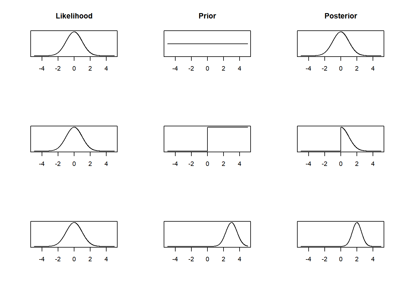

The posterior distribution is proportional to the likelihood function. The prior distribution closely matches frequentist inference. Both the MLE and posterior mean are 0.
We get a lopsided posterior distribution, that is proportional to the likelihood function for positive values of \(\theta\), but is 0 for negative values of \(\theta\).
We get some sort of average of the likelihood function and the prior distribution. Had we collected more data, the posterior distribution would have been weighted toward the information from the likelihood function more.

Now we have a framework to make estimates about model parameters given observed data. We’re now going to go through three examples using different probability distributions to illustrate how Bayesian inference works in practice.

2.6 The Binomial Distribution

The first example we are going to go through is with the Binomial distribution.

Example 2.4 A social media company wants to determine how many of its users are bots. A software engineer collects a random sample of 200 accounts and finds that three are bots. She uses a Bayesian method to estimate the probability of an account being a bot. She labels the accounts with a 1 if they are a bot and 0 if there is are a real person. The set of account labels is given by \(\boldsymbol{y} = \{y_1, \ldots, y_{200}\}\) and the probability an account is a bot is \(\theta\). By Bayes’ theorem, we obtain the following, \[ p(\theta \mid \boldsymbol{y}) \propto p(\boldsymbol{y}\mid \theta) p(\theta). \]

Likelihood function \(p(\boldsymbol{y}\mid \theta)\). We observe 200 trials each with the same probability of success (denoted by \(\theta\)) and probability of failure (given by \(1-\theta\)). The Binomial distribution seems the most suitable way of modelling this. Therefore, the likelihood function is given by, \[ p(\boldsymbol{y}\mid \theta) = \begin{pmatrix} 200 \\ 3 \end{pmatrix} \theta^3(1-\theta)^{197}, \] assuming that any two accounts being a bot are independent of one another.

Prior distribution \(p(\theta)\). We now need to describe our prior beliefs about \(\theta\). We have no reason to suggest \(\theta\) takes any specific value, so we use a uniform prior distribution \(\theta \sim U[0, 1]\), where \(p(\theta) = 1\) for \(\theta \in [0, 1]\).

Posterior distribution \(p(\theta \mid \boldsymbol{y})\). We can now derive the posterior distribution up to proportionality \[ p(\theta \mid \boldsymbol{y}) \propto \theta^3(1-\theta)^{197}. \] This functional dependence on \(\theta\) identifies the \(p(\theta \mid \boldsymbol{y})\) is a Beta distribution. The PDF for the beta distribution with shape parameters \(\alpha\) and \(\beta\) is \[ p(x \mid \alpha, \beta) = \frac{\Gamma(\alpha + \beta)}{\Gamma(\alpha)\Gamma(\beta)}x^{\alpha - 1}(1-x)^{\beta - 1}. \] The posterior distribution is therefore \(\theta \mid \boldsymbol{y} \sim \textrm{Beta}(4, 198)\).

2.7 Reporting Conclusions from Bayesian Inference

In the previous example, we derived the posterior distribution \(\theta \mid \boldsymbol{y} \sim \textrm{Beta}(4, 198)\). But often, we want to share more descriptive information about our beliefs given the observed data. In this example, the posterior mean given the data is \(\frac{4}{198+4} = \frac{2}{101}\). That is to say given the data, we expect that for every 101 accounts, two to be bots. The posterior mode for \(\theta\) is \(\frac{3}{200}\) or 1.5%.

It is important to share the uncertainty about out beliefs. In a frequentist framework, this would be via a confidence interval. The Bayesian analogue is a credible interval.

Definition 2.8 A credible interval is a central interval of posterior probability which corresponds, in the case of a 100\((1-\alpha)\)% interval, to the range of values that capture 100\((1-\alpha)\)% of the posterior probability.

Example 2.5 The 95% credible interval for the Binomial example is given by

cred.int.95 <- qbeta(c(0.025, 0.975), 4, 198)
round(cred.int.95, 3)

## [1] 0.005 0.043

This says that we believe there is a 95% chance that the probability of an account being a bot lies between 0.005 and 0.043. This is a much more intuitive definition to the confidence interval, which says if we ran the experiment an infinite number of times and computed an infinite number of confidence intervals, 95% of them would contain the true value of \(\theta\).

2.8 The Exponential Distribution

Example 2.6 An insurance company want to estimate the time until a claim is made on a specific policy. They describe the rate at which claims come in by \(\lambda\). The company provides a sample of 10 months at which a claim was made \(\boldsymbol{y} = \{14, 10, 6, 7, 13, 9, 12, 7, 9, 8\}\). By Bayes’ theorem, the posterior distribution for \(\lambda\) is \[ p(\lambda \mid \boldsymbol{y}) \propto p(\boldsymbol{y} \mid \lambda) p(\lambda). \]

Likelihood function \(p(\boldsymbol{y} \mid \lambda)\). The exponential distribution is a good way of modelling lifetimes or the length of time until an event happens. Assuming all the claims are independent of one another, the likelihood function is given by \[\begin{align*} p(\boldsymbol{y} \mid \lambda) &= \prod_{i=1}^{10} \lambda e^{-\lambda y_i} \\ & = \lambda^{10}e^{-\lambda \sum_{i=1}^{10} y_i} \\ & = \lambda^{10} e^{-95\lambda}. \end{align*}\]

Prior distribution \(p(\lambda)\). As we are modelling a rate parameter, we know it must be positive and continuous. We decide to use an exponential prior distribution for \(\lambda\), but leave the choice of the rate parameter up to the insurance professionals at the insurance company. The prior distribution is given by \(\lambda \sim \textrm{Exp}(\gamma).\)

Posterior distribution \(p(\lambda \mid \boldsymbol{y})\). We now have all the ingredients to derive the posterior distribution. It is given by \[\begin{align*} p(\lambda \mid \boldsymbol{y}) &\propto \lambda^{10} e^{-95\lambda} \times e^{-\gamma\lambda} \\ & \propto \lambda^{10}e^{-(95 + \gamma)\lambda} \end{align*}\] The functional form tells us that the posterior distribution is a Gamma distribution. The PDF of a gamma random variable with shape \(\alpha\) and rate \(\beta\) is \[ p(x \mid \alpha, \beta) = \frac{\alpha^\beta}{\Gamma(\alpha)}x^{\alpha-1}e^{-\beta x}. \] The distribution of the rate of the claims given the observed data is \(\lambda \mid \boldsymbol{y} \sim \textrm{Gamma}(11, 95 + \gamma)\).

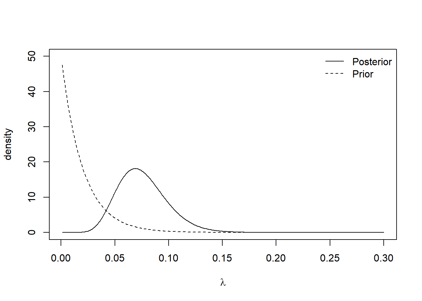
The posterior mean months until a claim is \(\frac{11}{95 + \gamma}\). We can see the effect of the choice of rate parameter in this mean. Small values of \(\gamma\) yield vague prior distribution, which plays a minimal role in the posterior distribution. Large values of \(\gamma\) result in prior distributions that contribute a lot to the posterior distribution. The plots below show the prior and posterior distributions for \(\gamma = 0.01\) and \(\gamma = 50\).

plot.distributions <- function(gamma.prior){
  #evaluate at selected values of lambda
  lambda <- seq(0.001, 0.3, 0.001) 
  
  #evaluate prior density
  prior <- dexp(lambda, rate = gamma.prior)
  
  #evaluate posterior density
  posterior <- dgamma(lambda, shape = 11, rate = 95 + gamma.prior)
  
  
  #plot
  plot(lambda, posterior, type= 'l', 
       ylim = c(0, 50), xlab = expression(lambda), ylab = "density")
  lines(lambda, prior, lty = 2)
  legend('topright', lty = c(1, 2), legend = c("Posterior", "Prior"),  
         bty = "n")
}

plot.distributions(0.01)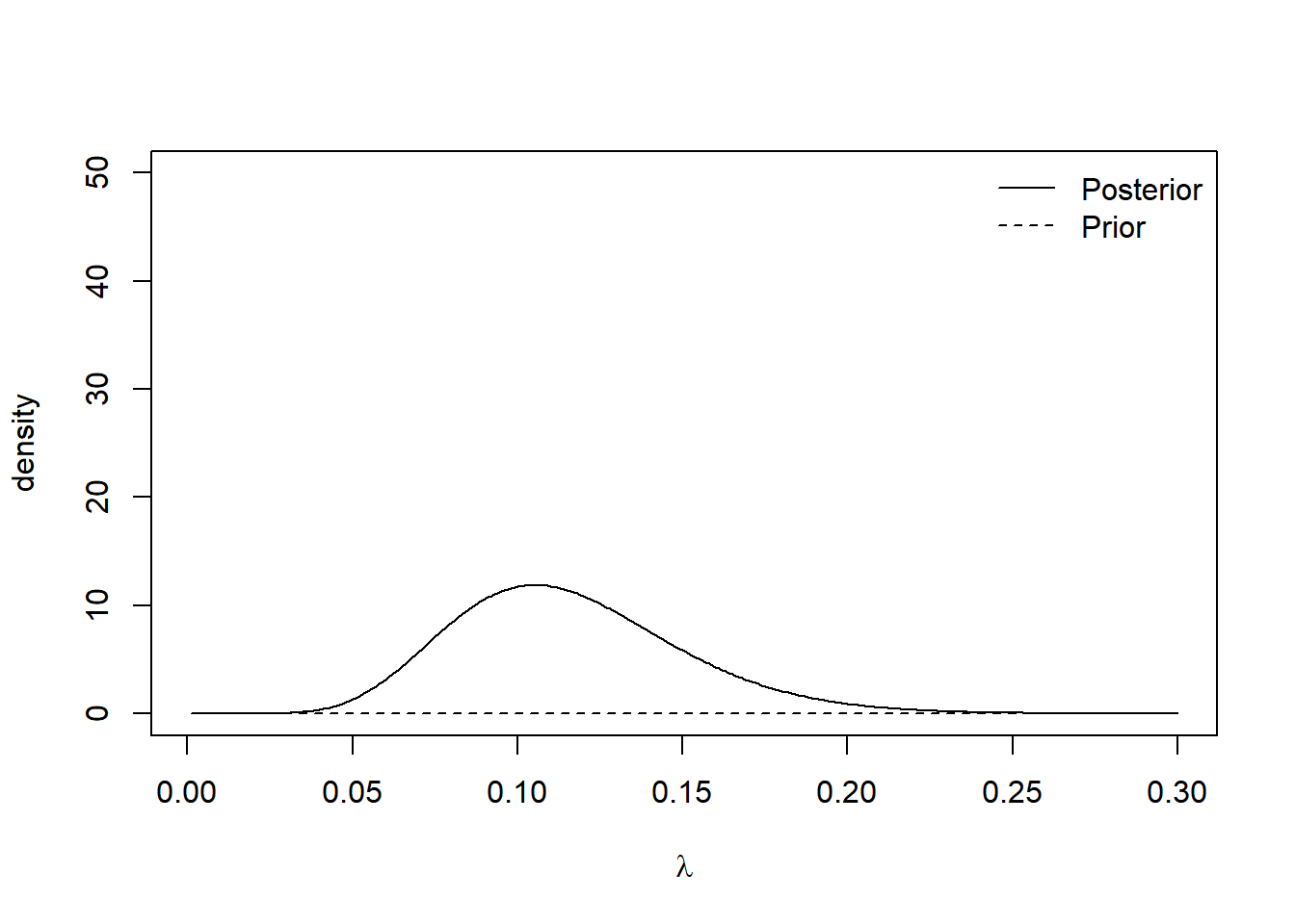

plot.distributions(50)

The insurance managers recommend that because this is a new premium, a vague prior distribution be used and \(\gamma = 0.01\). The posterior mean is \(\frac{11}{95.01} \approx 0.116\) and the 95% credible interval is

round(qgamma(c(0.025, 0.975), 11, 95.01), 3)

## [1] 0.058 0.194

2.9 The Normal Distribtuion

The Normal distribution is incredibly useful for modelling a wide range of natural phenomena and in its own right. We’re now going to derive posterior distributions for the normal distribution. As we’re going to see, the concepts behind deriving posterior distributions are the same as in the previous two examples. However, the algebraic accounting is a lot more taxing.

Example 2.7 Suppose we observe \(N\) data points \(\boldsymbol{y} = \{y_1, \ldots, y_N\}\) and we assume \(y_i \sim N(\mu, \sigma^2)\) and each observation is independent. Suppose that, somehow, we know the population standard deviation and we wish to estimate the population mean \(\mu\). By Bayes’ theorem, the posterior distribution is \[ p(\mu \mid \boldsymbol{y}, \sigma^2) \propto p(\boldsymbol{y} \mid \mu, \sigma^2) p(\mu) \]

Likelihood function. As the observations are independent, the likelihood function is given by the product of the \(N\) normal density functions as follows, \[\begin{align*} p(\boldsymbol{y} \mid \mu, \sigma^2) &= \prod_{i=1}^{N} \frac{1}{\sqrt{2\pi\sigma^2}}\exp\left\{-\frac{(y_i - \mu)^2}{2\sigma^2}\right\} \\ &= (2\pi\sigma^2)^{-\frac{N}{2}}\exp\left\{-\sum_{i=1}^{N}\frac{(y_i - \mu)^2}{2\sigma^2}\right\}. \end{align*}\]

Prior distribution We suppose we have no prior beliefs about the values that \(\mu\) can take. We assign a normal prior distribution to \(\mu \sim N(\mu_0, \sigma_0^2)\) despite it being a time. We will set \(\mu = 0\) and \(\sigma_0^2 = 1000\) to signify our vague prior beliefs, but, for ease, we will use the symbolic values during the derivation of the posterior distribution. We have \[ p(\mu) = \frac{1}{\sqrt{2\pi\sigma_0^2}}\exp\left\{-\frac{1}{2\sigma_0^2}(\mu - \mu_0)^2\right\}. \]

Posterior distribution. To derive the posterior distribution, up to proportionality, we multiply the prior distribution by the likelihood function. As the fractions out the front of both terms do not depend on \(\mu\), we can ignore these. \[\begin{align*} p(\mu \mid \boldsymbol{y}, \sigma^2) &\propto\exp\left\{-\sum_{i=1}^{N}\frac{(y_i - \mu)^2}{2\sigma^2}\right\} \exp\left\{\frac{1}{2\sigma_0^2}(\mu - \mu_0)^2\right\} \\ & = \exp\left\{-\sum_{i=1}^{N}\frac{(y_i - \mu)^2}{2\sigma^2}-\frac{1}{2\sigma_0^2}(\mu - \mu_0)^2\right\} \\ & = \exp\left\{-\frac{\sum_{i=1}^{N}y_i^2}{2\sigma^2} + \frac{\mu\sum_{i=1}^{N}y_i}{\sigma^2} - \frac{N\mu^2}{2\sigma^2} - \frac{\mu^2}{2\sigma_0^2} + \frac{\mu\mu_0}{\sigma_0^2} - \frac{\mu_0^2}{2\sigma_0^2}\right\}. \end{align*}\]

We can drop the first and last term as they do not depend on \(\mu\). With some arranging, the equation becomes \[ p(\mu \mid \boldsymbol{y}, \sigma^2) \propto \exp\left\{-\mu^2\left(\frac{N}{2\sigma^2} + \frac{1}{2\sigma_0^2}\right) + \mu\left(\frac{\sum_{i=1}^{N}y_i}{\sigma^2} + \frac{\mu_0}{\sigma_0^2} \right) \right\} \] Defining \(\mu_1 =\left(\frac{\sum_{i=1}^{N}y_i}{\sigma^2} + \frac{\mu_0}{\sigma_0^2} \right)\) and \(\sigma^2_1 = \left(\frac{N}{\sigma^2} + \frac{1}{\sigma_0^2}\right)^{-1}\) tidies this up and gives \[ p(\mu \mid \boldsymbol{y}, \sigma^2) \propto \exp\left\{-\frac{\mu^2}{2\sigma_1^2} + \mu\mu_1 \right\}. \] Our last step to turning this into a distribution is completing the square. Consider the exponent term, completing the square becomes \[ -2\sigma_1^2\mu^2 + \mu\mu_1 = -\frac{1}{2\sigma^2_1}\left(\mu - \frac{\mu_1}{\sigma_1^2} \right)^2. \] Therefore, the posterior distribution, up to proportionality, is given by \[ p(\mu \mid \boldsymbol{y}, \sigma^2) \propto \exp\left\{-\frac{1}{2\sigma^2_1}\left(\mu - \frac{\mu_1}{\sigma_1^2} \right)^2\right\}, \] and so the posterior distribution of \(\mu\) is \(\mu \mid \boldsymbol{y}, \sigma^2 \sim N(\mu_1, \sigma^2_1)\).

It may help to consider the meaning of \(\mu_1\) and \(\sigma^2_1\). The variance of the posterior distribution can be thought of as the weighted average of the population and sample precision, where the weight is the number of data points collected. The interpretation of the posterior mean can be seen more easily by writing is as \[ \mu = \sigma_1^2\left(\frac{N\bar{y}}{\sigma^2} + \frac{\mu_0}{\sigma_0^2} \right). \] The posterior mean is partially defined through the weighted average of the population and prior means, where the weighting depends on the number of data points collected and how precise the distributions are.

Now we have derived the posterior distribution, we can explore it using R. We simulate some data with \(N = 30\), \(\mu = 5\) and \(\sigma^2 = 1\).

#data
N <- 30
sigma <- 1
y <- rnorm(N, 5, sigma)

#prior
sigma0 <- 1000
mu0     <- 0

#posterior
sigma1.sq <- (1/(sigma0^2)  + N/(sigma^2))^-1
mu1       <- sigma1.sq*(sum(y)/(sigma^2) + mu0/(sigma0^2))

c(mu1, sigma1.sq) #output mean and variance

## [1] 4.97152974 0.03333333

#Create plot
mu <- seq(4, 6, 0.01)
posterior <- dnorm(mu, mean = mu1, sd = sqrt(sigma1.sq))
plot(mu, posterior, type ='l')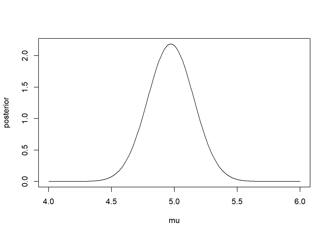

The 95% credible interval for the population’s mean reaction time is

qnorm(c(0.025, 0.975), mu1, sqrt(sigma1.sq))

## [1] 4.613691 5.329369

When the prior distribution induces the same function form in the posterior distribution, this is known as conjugacy.

Definition 2.9 If the prior distribution \(p(\theta)\) has the same distributional family as the posterior distribution \(p(\theta \mid \boldsymbol{y})\), then the prior distribution is a conjugate prior distribution.

2.10 Exercises

2.10.1 Conditional Probability

Consider a standard pack of 52 playing cards. You pick a card at random. What is the probability you pick:

A Queen, given you have picked a picture card (King, Queen, Jack)?
The five of clubs, given you have picked a black card?
A black card, given you have not picked the five of clubs?

Show answers

A pack of playing cards is equally divided into four suits: Hearts (red), Diamonds (red), Clubs (black), and Spades (black). Each suit has 13 cards numbered 2–10, Jack, Queen, King (the three picture cards), and Ace.

\[ p(\text{Queen} \mid \text{Picture}) = \frac{p(\text{Queen and Picture})}{p(\text{Picture})} = \frac{4/52}{12/52} = \frac{1}{3} \]
\[ p(\text{5 of Clubs} \mid \text{Black}) = \frac{p(\text{5 of Clubs and Black})}{p(\text{Black})} = \frac{1/52}{1/2} = \frac{1}{26} \]
\[ p(\text{Black} \mid \text{Not 5 of Clubs}) = \frac{p(\text{Black and Not 5 of Clubs})}{p(\text{Not 5 of Clubs})} = \frac{25/52}{51/52} = \frac{25}{51} \]

2.10.2 Frequentist vs Bayesian Probability

Decide if each of the following events can be assigned probabilities by frequentists:

The Bermuda Triangle exists.
Getting a 6 when rolling a die.
Someone will test positive for Covid-19 after contracting the disease.
The sun will rise tomorrow.

Show answers

No. This cannot be assigned a probability.
Yes. You can repeatedly roll dice, so a long-run frequency exists.
Yes. You can repeatedly test individuals for the disease, producing a long-run frequency of positive results.
It depends on what is meant by “tomorrow.”
- If “tomorrow” means a specific date (e.g., 2 January 2023), then no, since that date occurs only once.
- If “tomorrow” means “the day after today,” then yes, because there have been many such days over time, giving a long-run frequency.

2.10.3 Deriving Posterior Distribution

Suppose \(y_1, \ldots, y_N \sim \text{Geom}(p)\).
The density function for the Geometric distribution is

\[ p( y \mid p ) = (1-p)^{y - 1}p, \qquad p \in [0, 1], \, y \in \{1, 2, \ldots\} \]

Derive the likelihood function and then the maximum likelihood estimator for \(p\).
By letting \(p \sim \text{Beta}(\alpha, \beta)\), derive the posterior distribution for \(p\) given the data.

Show answers

The likelihood function is the product of the \(N\) geometric densities:
\[ p(\mathbf{y} \mid p) = \prod_{i=1}^N (1-p)^{y_i - 1}p = (1-p)^{\sum y_i - N}p^N. \]

The log-likelihood is
\[ \log p(\mathbf{y} \mid p) = (\sum y_i - N)\log(1-p) + N\log p. \]

Differentiating and setting to zero:
\[ -\frac{\sum y_i - N}{1-p} + \frac{N}{p} = 0 \] \[ \hat{p} = \frac{N}{\sum y_i}. \]

With prior \(p \sim \text{Beta}(\alpha, \beta)\),
\[ p(p) \propto p^{\alpha - 1}(1-p)^{\beta - 1}. \] Then the posterior is
\[ p(p \mid \mathbf{y}) \propto (1-p)^{\sum y_i - N}p^N \, p^{\alpha - 1}(1-p)^{\beta - 1} = p^{N + \alpha - 1}(1-p)^{\sum y_i - N + \beta - 1}. \] Thus,
\[ p \mid \mathbf{y} \sim \text{Beta}(N + \alpha, \, \sum y_i - N + \beta). \]

For each of the following statements, decide if they are true or false. Justify your answers.

The likelihood function is proportional to the posterior distribution.
A 99% credible interval captures 99% of the posterior probability.

Show answers

False. The posterior distribution is proportional to the product of the likelihood function and the prior distribution.
True. A 99% credible interval contains 99% of the posterior probability mass.

Let \(Y_1, \ldots, Y_N \sim \text{Pois}(\lambda)\).

Place a Gamma prior distribution on \(\lambda \sim \Gamma(\alpha, \beta)\) and derive the form the posterior distribution takes.
Fix \(\alpha = 1\). Discuss the effects of \(\beta\) on the posterior distribution.

Show answers

By Bayes’ theorem,
\[ p(\lambda \mid \mathbf{y}) \propto p(\mathbf{y} \mid \lambda)p(\lambda). \]

The likelihood is
\[ p(\mathbf{y} \mid \lambda) = \prod_{i=1}^N \frac{\lambda^{y_i} e^{-\lambda}}{y_i!} \propto \lambda^{\sum y_i} e^{-N\lambda}. \]

The prior is
\[ p(\lambda) = \frac{\beta^\alpha}{\Gamma(\alpha)} \lambda^{\alpha - 1} e^{-\beta \lambda}. \]

So
\[ p(\lambda \mid \mathbf{y}) \propto \lambda^{\sum y_i + \alpha - 1} e^{-(N + \beta)\lambda}. \]

Hence
\[ \lambda \mid \mathbf{y} \sim \Gamma\!\left(\sum_{i=1}^N y_i + \alpha, \, N + \beta\right). \]

With \(\alpha = 1\):
\[ \mathbb{E}(\lambda \mid \mathbf{y}) = \frac{\sum y_i + 1}{N + \beta}, \quad \mathrm{Var}(\lambda \mid \mathbf{y}) = \frac{\sum y_i + 1}{(N + \beta)^2}. \]

Small \(\beta\): prior weakly influences posterior.
Large \(\beta\): prior exerts stronger pull, reducing posterior mean and variance.