Chapter 5 Spatial Modelling with INLA

5.1 Motivation: Why Spatial Modelling?

In many social science applications, location matters. Whether you’re studying crime rates across neighborhoods, health outcomes across regions, or voting patterns across districts, the assumption that observations are independent often breaks down. Nearby areas tend to be more similar than distant ones—a phenomenon known as spatial autocorrelation.

Spatial modelling allows us to formally account for this dependence. By incorporating spatial structure into our models, we can:

Improve inference by borrowing strength from neighboring areas.
Avoid misleading conclusions that arise from ignoring spatial dependence.
Make better predictions for unobserved locations.
Identify spatial patterns that may reflect underlying social, economic, or environmental processes.

5.2 Why INLA?

Traditional Bayesian approaches to spatial modelling often rely on Markov Chain Monte Carlo (MCMC) methods, which can be computationally intensive and slow—especially for large datasets or complex models. INLA offers a fast and accurate alternative for latent Gaussian models, which include many commonly used spatial models.

INLA is particularly well-suited for: - Disease mapping - Ecological and environmental studies - Small area estimation - Policy evaluation across regions

In this session, we’ll use INLA to fit a simple spatial model using real-world data. The focus will be on hands-on implementation, so you can quickly see how you could implement spatial modelling.

To install INLA, run

install.packages("INLA",repos=c(getOption("repos"),INLA="https://inla.r-inla-download.org/R/stable"), dep=TRUE)
library(INLA)

## Loading required package: Matrix

## 
## Attaching package: 'Matrix'

## The following objects are masked from 'package:tidyr':
## 
##     expand, pack, unpack

## This is INLA_25.10.19 built 2025-10-19 19:10:20 UTC.
##  - See www.r-inla.org/contact-us for how to get help.
##  - List available models/likelihoods/etc with inla.list.models()
##  - Use inla.doc(<NAME>) to access documentation

5.3 Generalized Linear Mixed Models (GLMMs)

Social science data often exhibit hierarchical structure and unobserved heterogeneity. For example: - Students nested within schools - Patients nested within hospitals - Survey respondents nested within regions

In such cases, standard regression models may fail to capture the group-level variation or correlated errors. This is where Generalized Linear Mixed Models (GLMMs) come in.

GLMMs extend generalized linear models (GLMs) by including random effects, allowing us to: - Account for clustering in the data - Model variation across groups or units - Improve estimation and prediction by borrowing strength across levels

They are particularly useful when dealing with: - Binary outcomes (e.g., did someone vote?) - Count data (e.g., number of crimes in a district) - Repeated measures or longitudinal data

A Generalized Linear Mixed Model can be written as:

\[ g(\mathbb{E}[Y_i]) = \mathbf{x}_i^\top \boldsymbol{\beta} + \mathbf{z}_i^\top \mathbf{u} \]

Where:

\(Y_i\) is the response variable for observation \(i\) (e.g., count, binary outcome).
\(g(\cdot)\) is the link function (e.g., log for Poisson, logit for binomial).
\(\mathbf{x}_i\) is a vector of fixed effect covariates for observation \(i\).
\(\boldsymbol{\beta}\) is a vector of fixed effect coefficients.
\(\mathbf{z}_i\) is a vector of random effect covariates (often a subset of \(\mathbf{x}_i\)).
\(\mathbf{u}\) is a vector of random effects, typically assumed to follow a normal distribution: \[ \mathbf{u} \sim \mathcal{N}(0, \boldsymbol{\Sigma}) \]

This formulation allows us to model both population-level effects (via \(\boldsymbol{\beta}\)) and group-level variation (via \(\mathbf{u}\)), making GLMMs powerful tools for analyzing hierarchical or clustered data.

5.4 GLMMs and Spatial Modelling

In spatial contexts, GLMMs can incorporate spatially structured random effects to model dependence between nearby areas. This allows us to: - Capture spatial autocorrelation - Separate structured and unstructured variation - Make more accurate predictions for unobserved regions

GLMMs are a natural fit for Bayesian modelling, and tools like INLA make it easy to specify and fit these models efficiently.

In this session, we’ll use INLA to fit a GLMM with spatial random effects, exploring how to: - Specify fixed and random effects - Incorporate spatial structure - Interpret model outputs in a social science context

5.5 The Boston Housing Dataset

The Boston Housing dataset is a well-known dataset in statistics and machine learning, originally published by Harrison and Rubinfeld in 1978. It contains information on housing values in suburbs of Boston, along with a variety of socio-economic and environmental predictors.

Each observation corresponds to a census tract and includes variables

Variable	Description
TOWN	Town name
CMEDV	Corrected median of owner-occupied housing (in USD 1,000)
CRIM	Crime per capita
ZN	Proportion of residential land zoned for lots over 25,000 sq. ft per town
INDUS	Proportion of non-retail business acres per town
CHAS	Whether the tract borders the Charles River (1 = yes, 0 = no)
NOX	Nitric oxides concentration (in parts per 10 million)
RM	Average number of rooms per dwelling
AGE	Proportion of owner-occupied units built prior to 1940
DIS	Weighted distances to five Boston employment centres
RAD	Index of accessibility to radial highways per town
TAX	Full-value property-tax rate per USD 10,000 per town
PTRATIO	Pupil-teacher ratio per town
B	\(1000 \times (B_k - 0.63)^2\), where \(B_k\) is the proportion of Black residents
LSTAT	Percentage of lower status population

In social science, modelling house prices is useful for several reasons:

5.5.1 Understanding inequality

Housing prices reflect and reinforce socio-economic disparities. By modelling them, we can explore how factors like education, pollution, and crime relate to economic opportunity and social mobility.

5.5.2 Evaluating policy

Urban planners and policymakers use housing data to assess the impact of interventions such as zoning regulations, school funding, or transport infrastructure on affordability and access.

5.5.3 Capturing spatial dependence

House prices are spatially correlated: homes in nearby areas tend to have similar values due to shared amenities, environmental conditions, and demographic characteristics. This makes the dataset ideal for exploring spatial modelling techniques.

5.5.4 Making predictions

Accurate prediction of housing prices is valuable for real estate markets, taxation, and social planning. Bayesian methods allow us to quantify uncertainty in these predictions, which is crucial for informed decision-making.

5.6 Loading the Boston Housing Dataset in R

To begin working with the Boston Housing dataset, we first need to load it into our R session. The dataset is available in the spData package, which is widely used for spatial modelling. To work with spatial data in R, we use the sf package, which provides a modern and consistent framework for handling geospatial data.

# Load the required libraries
library(spData)

## To access larger datasets in this package, install the spDataLarge
## package with: `install.packages('spDataLarge',
## repos='https://nowosad.github.io/drat/', type='source')`

library(spdep)

## Loading required package: sf

## Linking to GEOS 3.13.1, GDAL 3.11.4, PROJ 9.7.0; sf_use_s2() is TRUE

library(sf)

data(boston)

boston <- sf::st_read(system.file("shapes/boston_tracts.gpkg",
                                     package="spData")[1])

## Reading layer `boston_tracts' from data source 
##   `C:\Users\joesm\AppData\Local\R\win-library\4.5\spData\shapes\boston_tracts.gpkg' 
##   using driver `GPKG'
## Simple feature collection with 506 features and 36 fields
## Geometry type: POLYGON
## Dimension:     XY
## Bounding box:  xmin: -71.52311 ymin: 42.00305 xmax: -70.63823 ymax: 42.67307
## Geodetic CRS:  NAD27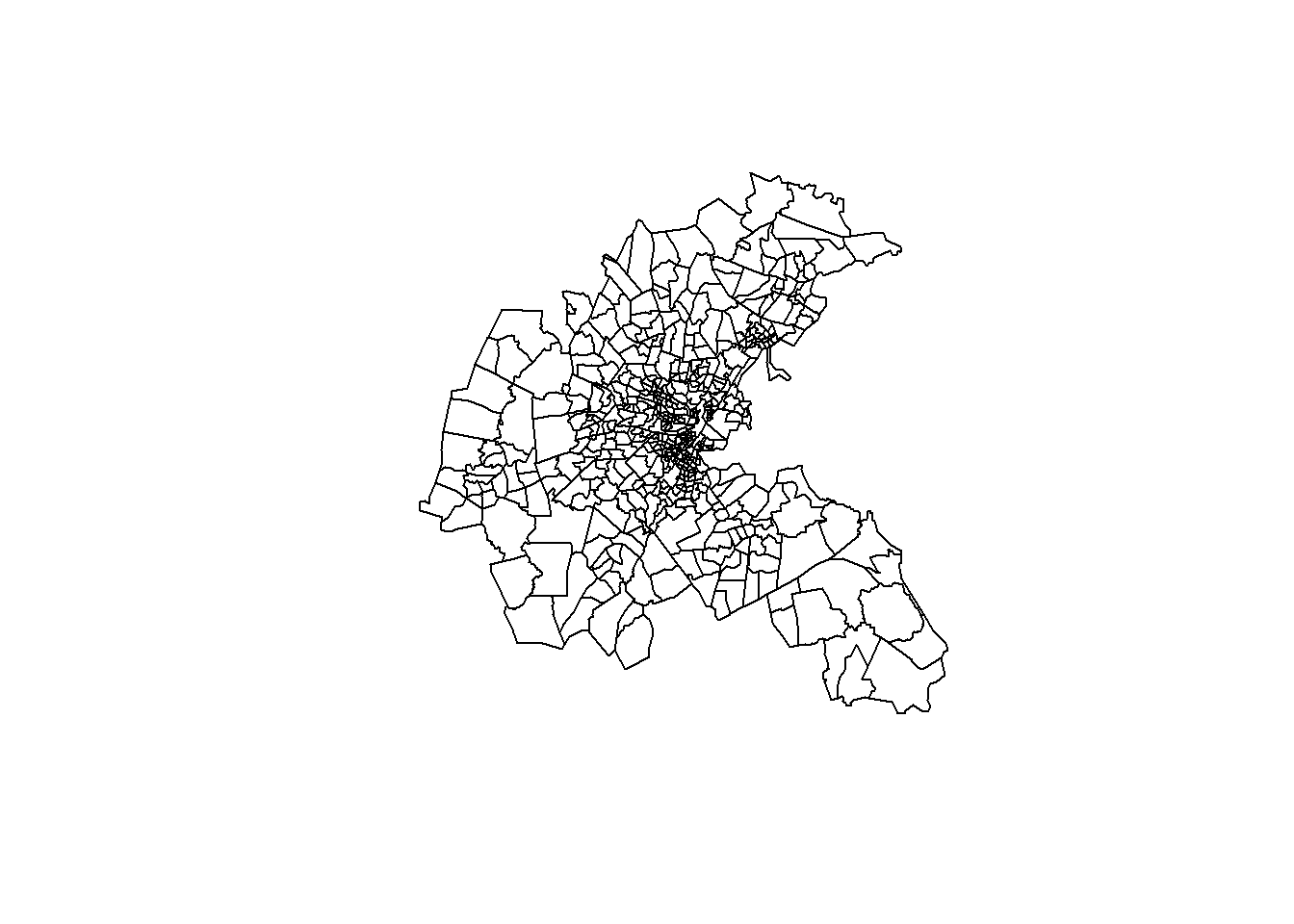

plot(boston$geom)

head(boston)

## Simple feature collection with 6 features and 36 fields
## Geometry type: POLYGON
## Dimension:     XY
## Bounding box:  xmin: -71.1753 ymin: 42.33 xmax: -71.1238 ymax: 42.3737
## Geodetic CRS:  NAD27
##   poltract                    TOWN TOWNNO TRACT      LON     LAT MEDV CMEDV
## 1     0001 Boston Allston-Brighton     74     1 -71.0830 42.2172 17.8  17.8
## 2     0002 Boston Allston-Brighton     74     2 -71.0950 42.2120 21.7  21.7
## 3     0003 Boston Allston-Brighton     74     3 -71.1007 42.2100 22.7  22.7
## 4     0004 Boston Allston-Brighton     74     4 -71.0930 42.2070 22.6  22.6
## 5     0005 Boston Allston-Brighton     74     5 -71.0905 42.2033 25.0  25.0
## 6     0006 Boston Allston-Brighton     74     6 -71.0865 42.2100 19.9  19.9
##      CRIM ZN INDUS CHAS  NOX    RM  AGE    DIS RAD TAX PTRATIO      B LSTAT
## 1 8.98296  0  18.1    1 0.77 6.212 97.4 2.1222  24 666    20.2 377.73 17.60
## 2 3.84970  0  18.1    1 0.77 6.395 91.0 2.5052  24 666    20.2 391.34 13.27
## 3 5.20177  0  18.1    1 0.77 6.127 83.4 2.7227  24 666    20.2 395.43 11.48
## 4 4.26131  0  18.1    0 0.77 6.112 81.3 2.5091  24 666    20.2 390.74 12.67
## 5 4.54192  0  18.1    0 0.77 6.398 88.0 2.5182  24 666    20.2 374.56  7.79
## 6 3.83684  0  18.1    0 0.77 6.251 91.1 2.2955  24 666    20.2 350.65 14.19
##   units cu5k c5_7_5 C7_5_10 C10_15 C15_20 C20_25 C25_35 C35_50 co50k median  BB
## 1   126    3      3       4     26     43     29     16      1     1  17800 0.8
## 2   399    4     10       7     37     95    139     93      9     5  21700 1.4
## 3   368    3      1       2     25     84    127    102     24     0  22700 0.3
## 4   220    3      2       2     23     45     67     63     12     3  22600 0.8
## 5    44    0      0       1      1     11      9     12      9     1  25000 1.8
## 6   221    2      3       7     31     69     72     30      6     1  19900 3.7
##   censored NOX_ID  POP                           geom
## 1       no      1 3962 POLYGON ((-71.1238 42.3689,...
## 2       no      1 9245 POLYGON ((-71.1546 42.3573,...
## 3       no      1 6842 POLYGON ((-71.1685 42.3601,...
## 4       no      1 8342 POLYGON ((-71.15391 42.3461...
## 5       no      1 7836 POLYGON ((-71.1479 42.337, ...
## 6       no      1 9276 POLYGON ((-71.1382 42.3535,...

boston$TRACT <- 1:506 #For our purposes, relabel census tracts in numerical order

We can now look at some histograms of the data:

# Single variable histogram
hist(boston$CMEDV,
     breaks = 20,
     col = "lightblue",
     main = "Median Home Value (MEDV)",
     xlab = "Value ($1000s)")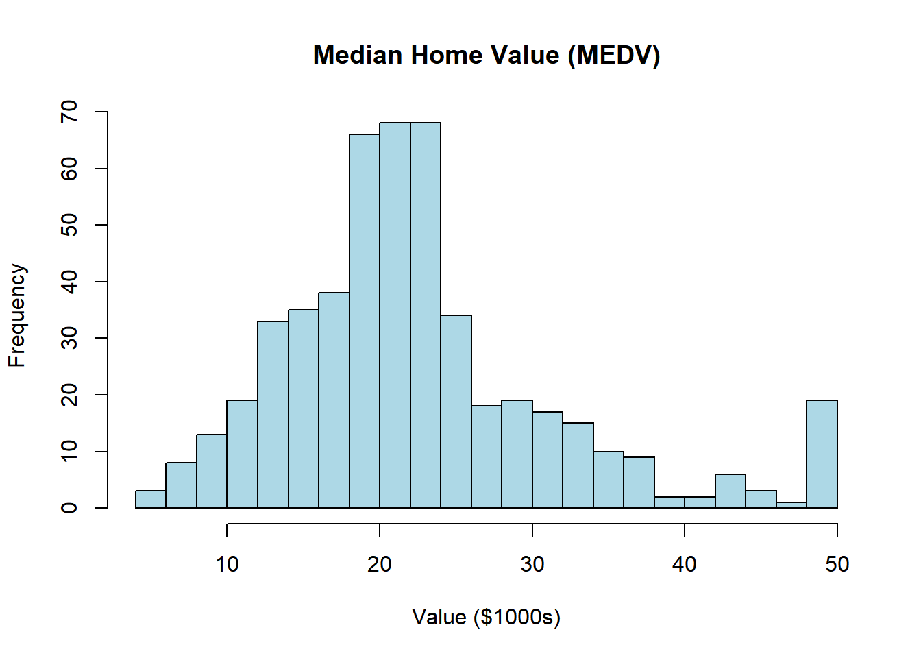

# Another variable
hist(boston$RM,
     breaks = 20,
     col = "orange",
     main = "Average Rooms per Dwelling (RM)",
     xlab = "Number of Rooms")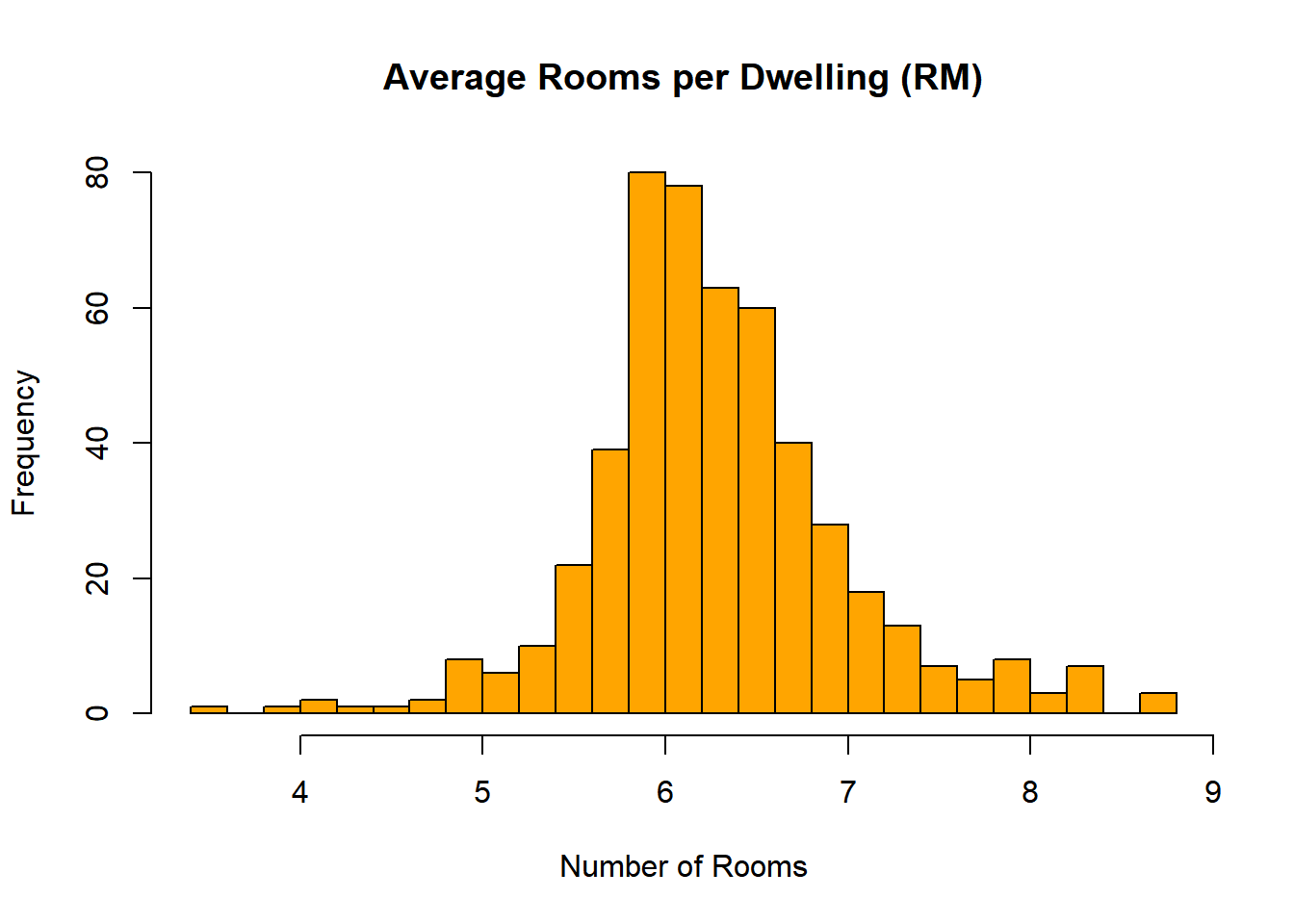

# Multiple histograms in one window
par(mfrow = c(2, 2))  # 2x2 grid

hist(boston$AGE, breaks = 20, col = "grey", main = "Proportion Built Before 1940", xlab = "AGE")
hist(boston$DIS, breaks = 20, col = "lightgreen", main = "Distance to Employment Centres", xlab = "DIS")
hist(boston$TAX, breaks = 20, col = "lightpink", main = "Property Tax Rate", xlab = "TAX")
hist(boston$NOX, breaks = 20, col = "lightyellow", main = "NO2 Particulate", xlab = "CRIM")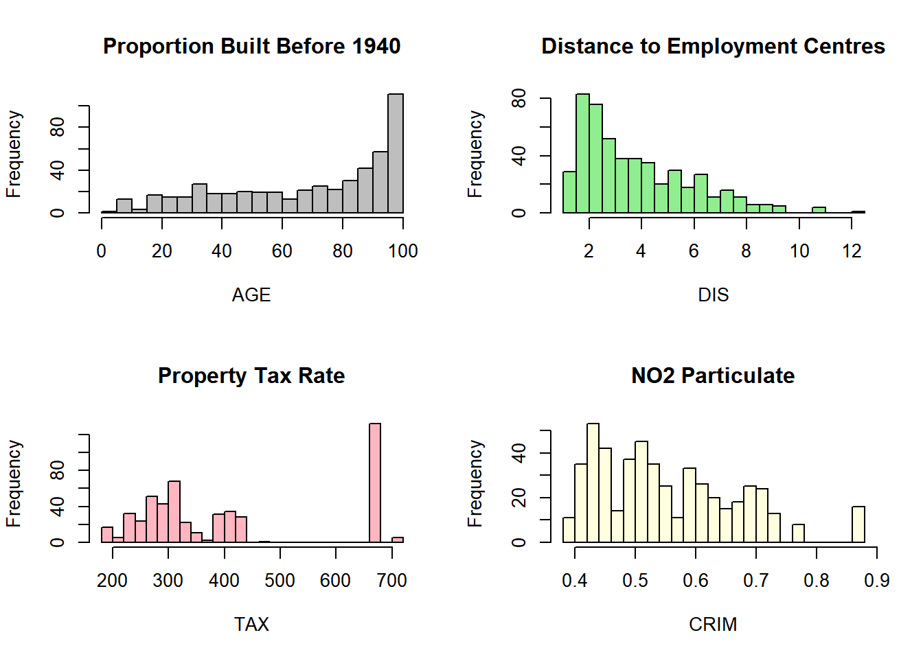

5.7 Specifying a Regression Model for Housing Prices

To explore the relationship between housing prices and socio-economic factors, we define a regression model using the Boston Housing dataset. The response variable is the log-transformed (corrected) median value of owner-occupied homes (CMEDV2), which helps stabilize variance and interpret effects multiplicatively.

We specify the model as in the original paper:

boston.form <- log(CMEDV) ~ CRIM + ZN + INDUS + CHAS + I(NOX^2) + I(RM^2) +
  AGE + log(DIS) + log(RAD) + TAX + PTRATIO + B + log(LSTAT)

Here, we are assuming the This formula includes a mix of linear and transformed predictors:

CRIM, ZN, INDUS, CHAS, AGE, TAX, PTRATIO, and B are included as linear terms.
NOX and RM are squared to capture potential non-linear effects.
DIS, RAD, and LSTAT are log-transformed to reduce skewness and improve model fit.

To account for unobserved heterogeneity across census tracts, we extend our regression model by including a random effect for each tract. This allows the model to capture tract-specific variation that is not explained by the observed covariates.

We use the INLA package to fit the model, specifying an IID (independent and identically distributed) random effect for the TRACT variable. This assumes that each tract (or area) has its own random variation, drawn from a common distribution.

The model is specified and fitted as follows:

boston.iid <- inla(
  update(boston.form, . ~ . + f(TRACT, model = "iid")),
  data = as.data.frame(boston),
  control.compute = list(dic = TRUE, waic = TRUE),
  control.predictor = list(compute = TRUE)
)

# View a summary of the fitted model
summary(boston.iid)

## Time used:
##     Pre = 0.544, Running = 0.727, Post = 0.137, Total = 1.41 
## Fixed effects:
##               mean    sd 0.025quant 0.5quant 0.975quant   mode kld
## (Intercept)  4.562 0.152      4.264    4.562      4.861  4.562   0
## CRIM        -0.012 0.001     -0.014   -0.012     -0.009 -0.012   0
## ZN           0.000 0.000     -0.001    0.000      0.001  0.000   0
## INDUS        0.000 0.002     -0.004    0.000      0.005  0.000   0
## CHAS1        0.092 0.033      0.028    0.092      0.156  0.092   0
## I(NOX^2)    -0.637 0.111     -0.856   -0.637     -0.419 -0.637   0
## I(RM^2)      0.006 0.001      0.004    0.006      0.009  0.006   0
## AGE          0.000 0.001     -0.001    0.000      0.001  0.000   0
## log(DIS)    -0.198 0.033     -0.262   -0.198     -0.133 -0.198   0
## log(RAD)     0.090 0.019      0.053    0.090      0.127  0.090   0
## TAX          0.000 0.000     -0.001    0.000      0.000  0.000   0
## PTRATIO     -0.030 0.005     -0.039   -0.030     -0.020 -0.030   0
## B            0.000 0.000      0.000    0.000      0.001  0.000   0
## log(LSTAT)  -0.375 0.025     -0.423   -0.375     -0.327 -0.375   0
## 
## Random effects:
##   Name     Model
##     TRACT IID model
## 
## Model hyperparameters:
##                                          mean   sd 0.025quant 0.5quant
## Precision for the Gaussian observations 51.18 4.65      42.91    50.88
## Precision for TRACT                     80.16 7.32      67.28    79.65
##                                         0.975quant  mode
## Precision for the Gaussian observations      61.20 50.09
## Precision for TRACT                          96.04 78.24
## 
## Deviance Information Criterion (DIC) ...............: -434.34
## Deviance Information Criterion (DIC, saturated) ....: 707.45
## Effective number of parameters .....................: 199.29
## 
## Watanabe-Akaike information criterion (WAIC) ...: -379.86
## Effective number of parameters .................: 196.28
## 
## Marginal log-Likelihood:  16.46 
##  is computed 
## Posterior summaries for the linear predictor and the fitted values are computed
## (Posterior marginals needs also 'control.compute=list(return.marginals.predictor=TRUE)')

This code does the fits a model using prior distributions and uses the following settings: - update(boston.form, . ~ . + f(TRACT, model = "iid")): Adds a random effect for each tract using the f() function. The “iid” model assumes that tract effects are independent and normally distributed. - data = as.data.frame(boston.tr): Converts the spatial data to a standard data frame for INLA. - control.compute: Requests computation of model fit statistics such as DIC (Deviance Information Criterion) and WAIC (Watanabe-Akaike Information Criterion). - control.predictor: Ensures that fitted values are computed and returned.

5.8 Fitting a Spatial Model with Besag-York-Mollié (BYM)

The Besag-York-Mollié (BYM) model is a popular approach for modelling spatially correlated random effects in spatial data. It is especially useful when observations are grouped by geographic regions, such as census tracts or wards, and we suspect that nearby areas may influence each other.

The BYM model decomposes spatial variation into two components:

Structured spatial effect: captures dependence between neighboring areas (i.e., spatial autocorrelation).
Unstructured spatial effect: captures random noise or variation that is not spatially correlated.

This allows us to model both the smooth spatial trends and the local, independent variation in the data.To fit a BYM model in INLA, we first need to define the neighborhood structure of the spatial units. This is done using the spdep package:

# Create adjacency list from polygon geometry
boston.adj <- poly2nb(boston$geom)

# Convert adjacency list to a binary adjacency matrix
W.boston <- nb2mat(boston.adj, style = "B")

Next, we can specify and fit the BYM model using INLA. The model includes both structured and unstructured random effects for the spatial units:

boston.bym <- inla(update(boston.form, . ~. +
    f(TRACT, model = "bym", graph = W.boston)), 
  data = as.data.frame(boston),
  control.compute = list(dic = TRUE, waic = TRUE),
  control.predictor = list(compute = TRUE)
)

# View model summary
summary(boston.bym)

## Time used:
##     Pre = 0.42, Running = 0.931, Post = 0.182, Total = 1.53 
## Fixed effects:
##               mean    sd 0.025quant 0.5quant 0.975quant   mode kld
## (Intercept)  3.861 0.165      3.538    3.861      4.184  3.861   0
## CRIM        -0.007 0.001     -0.010   -0.007     -0.005 -0.007   0
## ZN           0.000 0.000     -0.001    0.000      0.001  0.000   0
## INDUS       -0.001 0.002     -0.005   -0.001      0.004 -0.001   0
## CHAS1       -0.017 0.031     -0.077   -0.017      0.043 -0.017   0
## I(NOX^2)    -0.498 0.138     -0.770   -0.498     -0.227 -0.498   0
## I(RM^2)      0.009 0.001      0.007    0.009      0.012  0.009   0
## AGE         -0.001 0.001     -0.002   -0.001      0.000 -0.001   0
## log(DIS)    -0.190 0.068     -0.325   -0.190     -0.056 -0.190   0
## log(RAD)     0.055 0.020      0.015    0.055      0.095  0.055   0
## TAX          0.000 0.000     -0.001    0.000      0.000  0.000   0
## PTRATIO     -0.015 0.005     -0.025   -0.015     -0.004 -0.015   0
## B            0.001 0.000      0.000    0.001      0.001  0.001   0
## log(LSTAT)  -0.262 0.023     -0.307   -0.262     -0.218 -0.262   0
## 
## Random effects:
##   Name     Model
##     TRACT BYM model
## 
## Model hyperparameters:
##                                             mean       sd 0.025quant 0.5quant
## Precision for the Gaussian observations 22865.68 31330.17    1177.81 13109.56
## Precision for TRACT (iid component)       356.43   218.48     130.40   298.66
## Precision for TRACT (spatial component)    13.66     2.24       9.38    13.61
##                                         0.975quant    mode
## Precision for the Gaussian observations  103423.17 3041.18
## Precision for TRACT (iid component)         940.84  215.38
## Precision for TRACT (spatial component)      18.12   13.79
## 
## Deviance Information Criterion (DIC) ...............: -2830.55
## Deviance Information Criterion (DIC, saturated) ....: 1075.19
## Effective number of parameters .....................: 569.18
## 
## Watanabe-Akaike information criterion (WAIC) ...: -2862.75
## Effective number of parameters .................: 423.48
## 
## Marginal log-Likelihood:  220.80 
##  is computed 
## Posterior summaries for the linear predictor and the fitted values are computed
## (Posterior marginals needs also 'control.compute=list(return.marginals.predictor=TRUE)')

The BYM model allows us to account for spatial autocorrelation in housing prices. This means that the model can detect patterns where prices in one tract are influenced by prices in neighboring tracts. It improves inference and prediction by borrowing strength across space.

5.9 Plotting The Results

Once the BYM model has been fitted using INLA, we can extract and visualize the tract-level spatial random effects.

# Extract tract-level random effects
tract_effects <- boston.bym$summary.random$TRACT$mean[1:506]

# Set up color palette
palette <- colorRampPalette(c("green", "yellow", "blue"))
colors <- palette(10)

# Create color breaks
breaks <- cut(tract_effects, breaks = 10, labels = FALSE)

# Plot the spatial data
plot(st_geometry(boston), col = colors[breaks], main = "Spatial Random Effects (BYM Model)")

legend("bottomleft", legend = round(range(tract_effects[1:506]), 2),
       fill = c(colors[1], colors[10]), title = "Effect Range")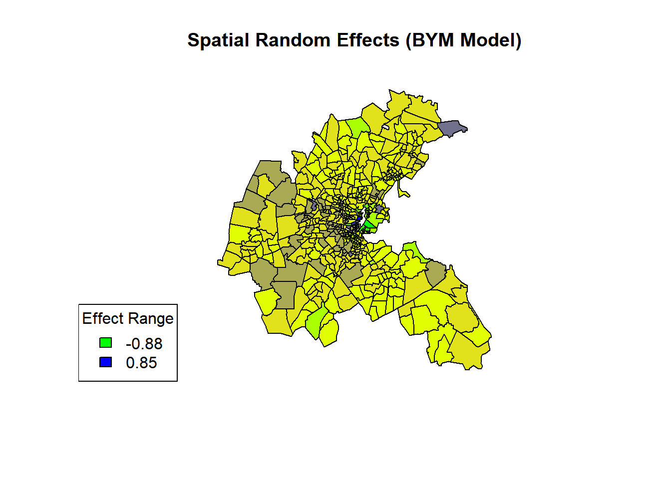

We can see the city centre has higher random effects, indicating higher housing prices after accounting for covariates. The spatial pattern reflects underlying socio-economic factors influencing housing values across Boston.